ELISA: Results - Quantitative, Qualitative and Sensitivity

s

The ELISA assay yields three different types of data output:

Quantitative

ELISA data can be interpreted in comparison to a standard curve (a serial dilution of a known, purified antigen) in order to precisely calculate the concentrations of antigen in various samples (Figure 6).

Qualitative

ELISAs can also be used to achieve a yes or no answer indicating whether a particular antigen is present in a sample, as compared to a blank well containing no antigen or an unrelated control antigen.

Semi-quantitative

ELISAs can be used to compare the relative levels of antigen in assay samples, since the intensity of signal will vary directly with antigen concentration.

Standard curve

ELISA data is typically graphed with optical density vs log concentration to produce a sigmoidal curve as shown in Figure 6. Known concentrations of antigen are used to produce a standard curve and then this data is used to measure the concentration of unknown samples by comparison to the linear portion of the standard curve. This can be done directly on the graph or with curve fitting software which is typically found on ELISA plate readers.

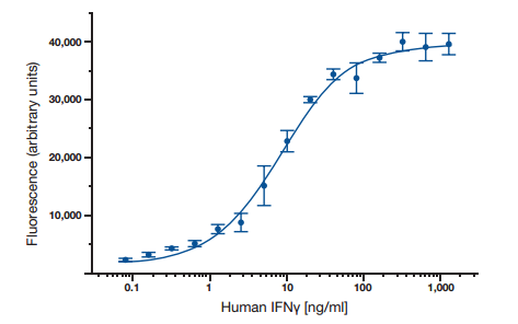
Fig. 6. A typical ELISA standard curve.

Calibration curve models

If a quantitative result is needed, the simplest way to proceed is to average the triplicate of the standards readings and deduct the reading of the blank control sample. Next, plot the standard curve, find the line of best fit or at least draw a point to point curve so that the concentration of the samples can be determined. Any dilutions made need to be adjusted for at this stage. This is generally the practical extent to which manual calculation can be taken.

A variation is to plot the data using semi-log, log/log, log/logit and its derivatives - the 4 or 5 parameter logistic models. Using software based/automated solutions makes it possible to consider more sophisticated graphing approaches. Using linear regression within a software package adds several more checking possibilities; it is possible to check the R2 value to determine overall goodness of fit. For that portion of the curve where the relationship of concentration to readout has a linear relationship, R2 values >0.99 represent a very good fit. Accuracy can then be further enhanced by using further standard concentrations in that range.

One aspect of the linear plot is that it compresses the data points on the lower concentrations of the standard curve, hence making that the most accurate range (area most likely to achieve the required R2 value). To counteract this compression a semi-log chart can be used; here the log of the concentration value (on x-axis) is plotted against the readout (on y-axis). This method gives an S-shaped data curve that distributes more of the data points into the more user friendly sigmoidal pattern.

The log/log (log of concentration against log of readout) plot type manages to linearize more of the data curve. The low to medium standard concentration range is generally linear in this model, only the higher end of the range tends to slope off. The log/logit and its derivatives, the 4 or 5 parameter logistic models, are more sophisticated requiring more complex calculations and estimations of max, min, EC50, and slope values. The 5 parameter model additionally requires the asymmetry value.

While these calibration curve models can deliver improved performance, a good starting point would be using the log-log plot with a check on the recovery percentage (analyte recovery from spiked samples). Alternatively, at least ‘back-fitting’ the standard curve readout values, is frequently ‘a good enough’ approach. The simplest way to check is to back calculate the calibration standards and check that they fall within 20% of the nominal readout value. One caveat is not to rely on ‘good’ R2 values and find that calibration curve model that delivers the best recovery values for the standards.

ELISA Sensitivity

ELISAs are one of the most sensitive immunoassays available. The typical detection range for an ELISA is 0.1 to 1 fmole or 0.01 ng to 0.1 ng, with sensitivity dependent upon the particular characteristics of the antibody-antigen interaction. In addition, some substrates such as those yielding enhanced chemiluminescent or fluorescent signal, can be used to improve results.

​As mentioned earlier, indirect detection will produce higher levels of signal and should therefore be more sensitive. However, it can also cause higher background signal thus reducing net specific signal levels.